Brownian Motion for Mathematical Finance
A simple introduction for basic knowledge on Brownian Motion and stochastic differential equation of Mathematical Finance.
Introduction
According to Wikipedia, Brownian motion, or Weiner Process, is the random motion of particles suspended in a medium (a liquid or a gas). But how do we apply these “physic-like” phenomena in the realm of Mathematical Finance?
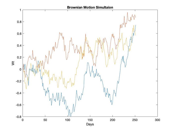
The answer is quite obvious, we can describe the price of stocks or assets as a Brownian Motion, which is a stimulation of the stochastic process under continuous time. To deal with some pricing theorem and hedging methodology, understanding the basic concept of Brownian Motion is extremely important.
Brownian Motion describe the stochasticity of price
Normal Distribution
Before carrying on to the topic, I have to explain an important concept — Normal Distribution. But, if you are familiar with it, feel free to skip this section.
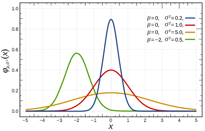
I believe most people have heard of normal distribution. To put it simply, normal distribution describes the distribution of many nature or social science experiments, including the distribution of the stock price in the future. The normal distribution looks like the following picture. The horizontal axis shows the variable x and the verticle axis describes the density (number) of the sample with given x.

As you can notice, there are two parameters controlling normal distribution — µ and σ². µ simply means the mean of this distribution, with larger µ, the curve peek will shift to the right. And with larger σ², the curve will stretch out more, namely, the data will be more scattered. So, to describe the distribution, we use the notation N(µ, σ²).
Central Limit Theorem is also an important theorem for normal distribution. It stated that when a large number of independent random variables (outcomes) are added, they tend to sum as a Normal Distribution. For example, when X ~ Distribution(µ, σ²), then ΣX ~ N(nµ, nσ²).
For more detailed information, you can refer to other articles or lecture videos from youtube. A good source will be Harvard Statistics lectures.
Brownian Motion
Definition: A random process {W(t): t ≥ 0} is a Brownian Motion (Wiener process) if the following conditions are fulfilled.

To convey it in a Financial scenario, let’s pretend we have an asset W whose accumulative return rate from time 0 to t is W(t). Suppose ∆t > 0 and is the unit time, then ∆W(t)=W(t+∆t) - W(t) means the return in time interval ∆t. We call the ∆W the increment, the return you got. Thus ∆W(t) means the increment at time t.
W(0)=0 as the first condition elaborated. Also, from condition 3 and 4 we know that ∆W(t)=W(t+∆t) - W(t) ~ N(0, ∆t) and each ∆W(t) is iid ~ N(0, ∆t). So, we can easily derive the following formula:

Let t = k * ∆t, then W(k) ~ N(0, k) = N(0, k*∆t) . We can also make k approaches infinity to make ∆t approaches 0. Thus, we can make this discrete model into a continuous one.
From the viewpoint of the continuous model, we can redefine the equation:

However, when we want to stimulate the stock price, we will use a discrete model and run simulations such as Monte Carlo or Binomial Tree.

However, to better stimulate Brownian Motion, we often use another method called Random Walk. So, let’s talk about Random Walk.
Also, if you wish to run a Monte Carlo yourself, I’ve made a simple program for you to give it a shot. GITHUB Link!
Random Walk
Besides using the discrete or continuous model of Brownian Motion, we can also use another technique called random walk. Random walk is derived from a series of rescaled Bernoulli Random Variables, we can use them to stimulate a Brownian Motion.
Random Walk is basically the standpoint for pricing models such as Binomial Tree. So, let’s define a Bernoulli random variable X. The outcome space of X is {1, -1} and the probability for each is p and 1-p.

Let’s define another random variable M. M is basically the cumulation of all previous X. Also, we perform X performs k time iid. Every X stands for a small price change, so M is basically the summation of all change, namely the price.

Since all X performed independently, we know that the difference between two different M is also independent. We call the difference between these M increments and the formula is as below.

The mean will be 0 and variance is k(i+1) - k(i). This can be easily computed with the Bernoulli distribution. To use the random walk to stimulate Brownian Motion, we still need to rescale M. So, here is how we do it. We define the rescaling version of M as W. The superscript n denotes the magnitude of our rescaling.

Since we make n really large, we can apply the central limit theorem. Also, by rescaling, we can make W(t) follows N(0, t). So, this is a tricky part and maybe you can try to go through it on your own.
There are a whole lot of topics to dig into, such as martingale and Markov Property, however, I will leave it to the future. You can also refer to other online sources if you wish so.
After knowing how to use the random walk to stimulate Brownian Motion, we are catching up on Ito Process. It is derived from Brownian Motion and can later be used to stimulate the movement of the market.

So, ΔX can be used to stimulate a broader increment with drift and rescale of W. The term rΔt is the drift and σΔW is the rescale of random walk. With X, we can depict a more complex increment. Also, we often make the delta infinitely small to make it continuous.

The dt term is often regarded as the drift term and dW as the martingale term. In the financial model, the coefficient of dt, which is r, is referred to the growth rate and the coefficient of dW is the volatility rate.
This is the stochastic differential equation (SDE).
It is the foundation of mathematic finance. The further application will be built with equations like this.
There is much more to be covered and SDE is only the start of mathematical finance. Hope you enjoy it! More will be covered in the near future.
Linked-in: www.linkedin.com/in/albert-hk-lin
GitHub: https://github.com/AlbertLin0327
